TensorFlow goes the JS Way — Getting Started — Episode #1

Its 5 in the morning here, and what keeps me awake is the newest kid in the JS town. Of all the amazing announcements in Today’s TF Dev summit, what made my day was Tensorflow.js. I am writing this to share my learnings with Tensorflow.js in last 6 hours.

Any application that can be written in JavaScript, will eventually be written in JavaScript.

~Jeff Atwood, co-founder StackOverflow

Installation

Tensorflow.js is available via NPM and CDN

You can simply do a npm installnpm install @tensorflow/tfjs

or call it via CDN like any other JS library

<script src="https://cdn.jsdelivr.net/npm/@tensorflow/tfjs@0.6.1"></script>

The official documentation uses ES8 syntax (async, await etc) and I will be following along.

Basics

Tensors

If you are familiar with TensorFlow you must be knowing tensors already. If you don't know it yet, nothing to worry about. It is a mathematical representation somewhat analogous to vectors, represented by an array of components that are functions of the coordinates of a space. Sounds difficult ?Don't worry this guy has you covered in this amazing video. Watch to understand what are tensors. Kudos to Mr. Dan Fleisch for this.

So as you may guess the central unit of data in TensorFlow.js is the tensor: a set of numerical values shaped into an array of one or more dimensions. A The shape of array of a Tensor instance is defined by an attribute of shape which defines the number of values in each dimension of the array.

The primary Tensor constructor is the tf.tensor function:// 2x3 Tensor
const shape = [2, 3];
// 2 rows, 3 columns const a = tf.tensor([1.0, 2.0, 3.0, 10.0, 20.0, 30.0], shape); a.print(); // print Tensor values // Output: [[1 , 2 , 3 ],
// [10, 20, 30]]

Tensorflow.js provides following functions for constructing low-rank tensors, to enhance code readability: tf.scalar, tf.tensor1d, tf.tensor2d, tf.tensor3d and tf.tensor4d. It also provides tf.zeros for all values set to 0 andtf.onesfor all values set to 1// 3x5 Tensor with all values set to 0
const zeros = tf.zeros([3, 5]);
// Output: [[0, 0, 0, 0, 0],
//           0, 0, 0, 0, 0],
//         [0, 0, 0, 0, 0]]

Note : In TensorFlow.js, tensors are immutable; once created, you cannot change their values. Instead you perform operations on them that generate new tensors.

Variables

Variables are initialized with a tensor of values. Unlike Tensors, however, their values are mutable. You can assign a new tensor to an existing variable using the assign method:const initialValues = tf.zeros([5]);
const biases = tf.variable(initialValues); // initialize biases
biases.print(); // output: [0, 0, 0, 0, 0]  const updatedValues = tf.tensor1d([0, 1, 0, 1, 0]); biases.assign(updatedValues); // update values of biases biases.print(); // output: [0, 1, 0, 1, 0]

Apart from these tensorflow.js has APIs for Ops(operations) and Models and Layers. Ops are functions like add(), sub(), mul() etc, to perform mathematical operations on tensors and Models and Layers are present to define models. Either we can create our function which takes an input and returns a predicted value and call it a model, or we can use inbuilt method called tf.model and use pre existing mathematical layer representations to achieve abstractions for Deep Learning.

Memory Management: dispose and tf.tidy

The very first question that I had when I saw the announcement for tensorflow.js was about memory. Its difficult to imagine all those GPU intensive algorithms running on browsers. This API from tensorflow.js has most of the answers, You can call dispose on a tensor or variable to purge it and free up its GPU memory. Where as tf.tidy executes a function and purges any intermediate tensors created, freeing up their GPU memory. It does not purge the return value of the inner function. It also does not clean the variables but we can always purge our variables by calling dispose.

You can see what happened when my friend Rahul Kumar tried running MNIST from the official examples. 763 MB sucked !. But this is just the beginning and this can be controlled by the proper use of dispose and tidy functions.

Let’s go through one of the sample projects from the official examples section.

Please note that this is step by step similar to whats documented at the official example section. I have made few changes but that broke the code, I will update my section of code soon.

Fitting a Curve to Synthetic Data

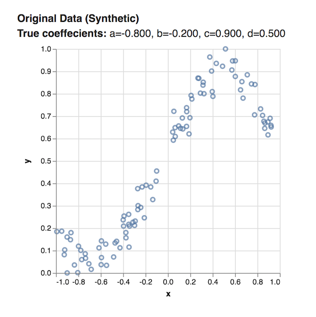
We have to fit a curve on this plot of dots which was generated using a cubic function of the format y = ax3 + bx2 + cx + d. That is our task is to learn the coefficients of this function: the values of a, b, c, and d that best fit the data

Step 1: Set up Variables

First, let’s create some variables to hold our current best estimate of these values at each step of model training. To start, we’ll assign each of these variables a random number:

const a = tf.variable(tf.scalar(Math.random()));const b = tf.variable(tf.scalar(Math.random()));const c = tf.variable(tf.scalar(Math.random()));const d = tf.variable(tf.scalar(Math.random()));

Step 2: Build a Model

We can represent our polynomial function y = ax3 + bx2 + cx + d in TensorFlow.js by chaining a series of mathematical operations: addition (add), multiplication (mul), and exponentiation (pow and square).

The following code constructs a predict function that takes x as input and returns y:

function predict(x) {  // y = a * x ^ 3 + b * x ^ 2 + c * x + d  return tf.tidy(() => {    return a.mul(x.pow(tf.scalar(3))) // a * x^3      .add(b.mul(x.square())) // + b * x ^ 2      .add(c.mul(x)) // + c      .add(d);  });}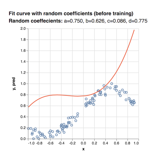

Since the points taken are random the graph does not fit at all to start with.

Step 3: Train the Model

Our final step is to train the model to learn good values for the coefficients. To train our model, we need to define three things:

• A loss function, which measures how well a given polynomial fits the data. The lower the loss value, the better the polynomial fits the data.
• An optimizer, which implements an algorithm for revising our coefficient values based on the output of the loss function. The optimizer’s goal is to minimize the output value of the loss function.
• A training loop, which will iteratively run the optimizer to minimize loss.

Define the Loss Function

For this tutorial, we’ll use mean squared error (MSE) as our loss function. MSE is calculated by squaring the difference between the actual y value and the predicted y value for each x value in our data set, and then taking the mean of all the resulting terms.

We can define a MSE loss function in TensorFlow.js as follows:

function loss(predictions, labels) {  // Subtract our labels (actual values) from predictions, square the results,  // and take the mean.  const meanSquareError = predictions.sub(labels).square().mean();  return meanSquareError;}

Define the Optimizer

TensorFlow.js providestf.train.sdg which takes as input a desired learning rate, and returns an SGDOptimizer object, which can be invoked to optimize the value of the loss function.

The learning rate controls how big the model’s adjustments will be when improving its predictions.

The following code constructs an SGD optimizer with a learning rate of 0.5:

const learningRate = 0.5;const optimizer = tf.train.sgd(learningRate);

Define the Training Loop

Now that we’ve defined our loss function and optimizer, we can build a training loop, which iteratively performs SGD to refine our model’s coefficients to minimize loss (MSE). Here’s what our loop looks like:

function train(xs, ys, numIterations = 75) {

  const learningRate = 0.5;  const optimizer = tf.train.sgd(learningRate);

  for (let iter = 0; iter < numIterations; iter++) {    optimizer.minimize(() => {      const predsYs = predict(xs);      return loss(predsYs, ys);    });  }}

First, we define our training function to take the x and y values of our dataset, as well as a specified number of iterations, as input:

function train(xs, ys, numIterations) {...}

Next, we define the learning rate and SGD optimizer as discussed in the previous section:

const learningRate = 0.5;const optimizer = tf.train.sgd(learningRate);

Finally, we set up a for loop that runs numIterations training iterations. In each iteration, we invoke minimizeon the optimizer, which is where the magic happens:

for (let iter = 0; iter < numIterations; iter++) {  optimizer.minimize(() => {    const predsYs = predict(xs);    return loss(predsYs, ys);  });}

minimize takes a function that does two things:

1. It predicts y values (predYs) for all the x values using the predict model function we defined earlier in Step 2.
2. It returns the mean squared error loss for those predictions using the loss function we defined earlier in Define the Loss Function.

minimize then automatically adjusts any variables used by this function (here, the coefficients a, b, c, and d) in order to minimize the return value (our loss).

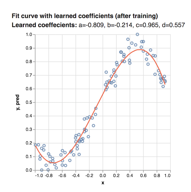
After running our training loop, a, b, c, and d will contain the coefficient values learned by the model after 75 iterations of SGD.

Results

Once the program runs through all the loops, the final values of a, b, c and d can be used to plot the curve.

I will be working on my experiments of ML with tensorflow.js over this weekend and will write about them in the second part of this series.